How to Use VLOOKUP in Google Sheets from Another Tab and Spreadsheet
Many users struggle to pull data from another tab or spreadsheet in Google Sheets. They try to match values manually or use formulas that do not work correctly. This makes the process slow and increases the chance of errors. Managing large datasets becomes difficult without the right method.
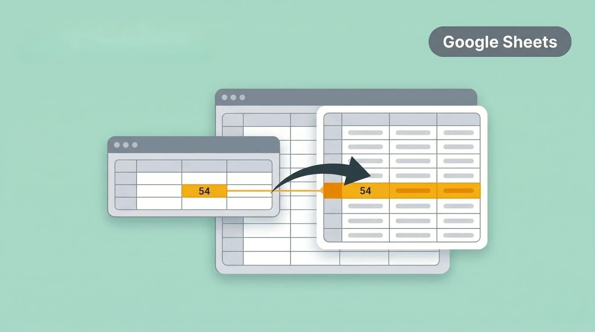
VLOOKUP helps you solve this problem by finding and retrieving data automatically. You can use it within the same sheet or across different spreadsheets. This makes data handling faster and more accurate. In this guide, you will learn how to use VLOOKUP step by step.
What Is VLOOKUP in Google Sheets
VLOOKUP is a function used to search for a value in a table. It looks for the value in the first column and returns matching data from another column. This helps you find information quickly without manual searching. It is useful when working with large datasets. The function works by scanning data vertically.
Once it finds the match, it pulls the related value from the specified column, saving time and reducing errors in data handling. VLOOKUP is commonly used for tasks like matching names, IDs, or product details. It helps you organize and analyze data more efficiently, especially when combined with pivot tables for deeper insights.
VLOOKUP Formula Syntax
VLOOKUP uses a simple formula structure in Google Sheets. You need to understand each part to use it correctly. This helps you avoid errors and get accurate results, especially when preparing data for Looker Studio reports.
The formula looks like this: VLOOKUP (search_key, range, index, [is_sorted])
Each part plays an important role in the result. Using the correct values ensures the formula works properly.
How to Use VLOOKUP from Another Tab
You can use VLOOKUP to pull data from another tab in Google Sheets. This helps you organize data across multiple sheets. You just need to reference the correct tab in your formula.
Step 1: Prepare Your Data
Make sure your data is properly organized in both tabs. The lookup value should exist in the first column of your table. Clean data helps avoid errors.
Step 2: Write the VLOOKUP Formula
Start writing the formula in the cell where you want the result. Enter the search value you want to match.
Step 3: Select Range from Another Tab
Use the tab name followed by an exclamation mark. For example: Sheet2!A:B. This tells Google Sheets to look in another tab.
Step 4: Apply the Formula
Complete the formula with the correct column index and FALSE for an exact match. Press enter to get the result. The value will be fetched from the other tab automatically.
How to Use VLOOKUP from Another Spreadsheet
You can also use VLOOKUP to pull data from a different spreadsheet in Google Sheets. For this, you need to use the IMPORTRANGE function. It allows you to connect two spreadsheets and access data.
Step 1: Use IMPORTRANGE
Start by using the IMPORTRANGE function to import data. You need the spreadsheet URL and the range. For example:
IMPORTRANGE(“spreadsheet_url”, “Sheet1!A:B”)
Step 2: Allow Access
The first time you use IMPORTRANGE, Google Sheets will ask for permission. Click Allow access to connect both spreadsheets.
Step 3: Combine with VLOOKUP
Now use VLOOKUP with IMPORTRANGE. Wrap IMPORTRANGE inside VLOOKUP as the range. This allows you to search and fetch data from another file. Once set up, your data will update automatically. This makes it easy to manage data across multiple spreadsheets.
Common Errors in VLOOKUP and Fixes
VLOOKUP can return errors if the formula is not set correctly in Google Sheets. These errors are common but easy to fix. Understanding them helps you use the function correctly.
#N/A Error
This error appears when the value is not found. It usually happens when the lookup value does not exist in the first column. Make sure your data matches exactly.
Wrong Range Selection
If you select the wrong range, VLOOKUP will return incorrect results. Always ensure the lookup column is the first column in your range. This is required for the function to work.
Incorrect Column Index
Using the wrong column number gives wrong data. The index should match the position of the column in your range. Double-check your column number.
Missing Exact Match
If you use TRUE instead of FALSE, results may be inaccurate. Always use FALSE for exact matches. This ensures correct data retrieval.
Best Practices for Using VLOOKUP
Using VLOOKUP correctly in Google Sheets helps you avoid errors and get accurate results. Small improvements in your setup can make a big difference, especially when working with campaign data that includes UTM parameters. Following best practices keeps your data clean and reliable.
Make sure your data is well organized before using VLOOKUP. Keep the lookup column on the left side of your table. Use clear and consistent data to avoid mismatches. This helps the function work properly.
Always use FALSE for an exact match to get accurate results. Double-check your column index and range selection. You can also use named ranges to make formulas easier to manage. These practices help you work faster and reduce errors.
Common Mistakes to Avoid
Many users make mistakes while using VLOOKUP in Google Sheets. These errors can return wrong results or no data at all. Most issues happen due to small mistakes in data setup or formula usage. You need to handle both carefully for accurate results.
Lookup Value Not in First Column
VLOOKUP only searches in the first column of your range. If your lookup value is in another column, the formula will not find it. Rearrange your data so the lookup column is first.
Using Approximate Match by Mistake
Using TRUE instead of FALSE can return incorrect results. TRUE works only with sorted data and may give wrong matches. Always use FALSE for exact and accurate results.
Incorrect Range Reference
Selecting the wrong range leads to errors or incorrect data. Make sure your selected range includes the lookup column and result column. Double-check your range before applying the formula.
Not Locking Range
When you copy the formula, the range may shift automatically. This can break your results. Use $ signs to lock the range and keep it fixed.
Ignoring Data Format Issues
VLOOKUP fails when data formats do not match. For example, text and numbers may look the same but are different. Make sure both the lookup value and the data use the same format.
Conclusion
VLOOKUP in Google Sheets helps you manage and analyze data efficiently. It allows you to fetch data from another tab or even another spreadsheet. This makes your workflow faster and more accurate. It also reduces manual effort and errors.
Use the correct formula structure and follow best practices. Avoid common mistakes and keep your data clean. Test your formulas to ensure accuracy. This approach helps you use VLOOKUP effectively and improve your data handling.